Set Theory and Probability I

October 25, 2025 Mathematics Probability Theory

This note presents fundamental concepts in Set Theory and Probability Theory. Material from CSE422 class (taught by Md. Shahriar Karim, Assistant Professor, North South University) lectures is enhanced with definitions, theorems, examples, and proofs from faculty notes [1][2] and textbooks by Ross [3] and Chan [4]. Topics include set operations, cardinality, probability spaces, axioms, corollaries, probability assignment (pmf/pdf), measure zero sets, and conditional probability.

Set Theory

Set theory forms the fundamental language and mathematical basis for understanding probability. We begin by defining the core concepts.

Sets and Elements

A set is a collection of distinct objects, considered as an entity in itself. The objects within the set are called its elements or members. Sets are typically denoted by capital letters (e.g., $A, B, S$) and their elements by lowercase letters or symbols.

Definition: Set

A set is a collection of distinct elements. We often denote a set by listing its elements within curly braces [1][4].

A = \{\xi_1, \xi_2, \ldots, \xi_n\}

where $\xi_i$ is the $i$-th element in the set.

Remark

The elements in a set are distinct (no repetitions) and unordered (the order in which elements are listed does not matter).

Example 1: Basic Sets

$A = \{2, 7, 9\}$ is a finite set of numbers.
$B = \{\text{apple, orange, pear}\}$ is a finite set of objects.
$C = \{2, 4, 6, 8, \ldots\}$ is an infinite set (the set of positive even integers).

Definition: Element Membership

If an object $\xi$ is an element of a set $A$, we write $\xi \in A$. If $\xi$ is not an element of $A$, we write $\xi \notin A$.

Describing Sets

Sets can be described explicitly by listing elements or implicitly using properties.

Definition: Set Builder Notation

A set can be defined by specifying a property that its elements must satisfy.

A = \{x \mid P(x)\}

This reads as "A is the set of all elements $x$ such that property $P(x)$ is true."

Example 2: Set Builder Notation

$A = \{1, 2, 3, 4, 5, 6, 7, 8, 9\}$ can be written as $A = \{x \mid x \in \mathbb{Z}^+ \text{ and } 1 \le x \le 9\}$.
The set of even integers can be written as $E = \{x \mid x = 2k \text{ for some integer } k\}$.

Fundamental Set Concepts

Definition: Set Equality

Two sets $A$ and $B$ are equal ($A = B$) if and only if they contain exactly the same elements [1][3].

Definition: Cardinality

The cardinality of a finite set $A$, denoted $|A|$, is the number of distinct elements in the set [1].

Example 3: Cardinality

For $A = \{2, 7, 9\}$, $|A| = 3$.

Definition: Universal Set ($\Omega$)

In a particular context, the Universal Set ($\Omega$ or $S$) is the set containing all possible elements under consideration [1][4].

Definition: Empty Set ($\emptyset$)

The Empty Set ($\emptyset$ or $\{\}$) is the unique set containing no elements [1][3].

Definition: Subset ($A \subseteq B$)

Set $A$ is a subset of set $B$ if every element of $A$ is also an element of $B$ [4]. If $A \subseteq B$ and $A \ne B$, then $A$ is a proper subset of $B$, denoted $A \subset B$.

Theorem 1: Set Equality via Subsets

Two sets $A$ and $B$ are equal if and only if $A \subseteq B$ and $B \subseteq A$ [4].

Set Operations

These operations allow us to combine or modify sets.

Definition: Union ($A \cup B$)

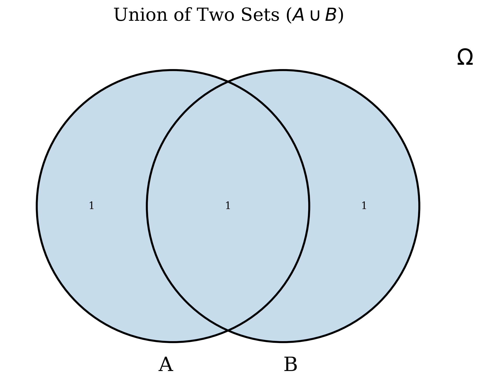
The union of sets $A$ and $B$ is the set containing all elements that are in $A$, or in $B$, or in both [3].

A \cup B = \{x \mid x \in A \text{ or } x \in B\}

Example 4: Union

If $A = \{1, 2, 3\}$ and $B = \{3, 4, 5\}$, then $A \cup B = \{1, 2, 3, 4, 5\}$.

Definition: Intersection ($A \cap B$)

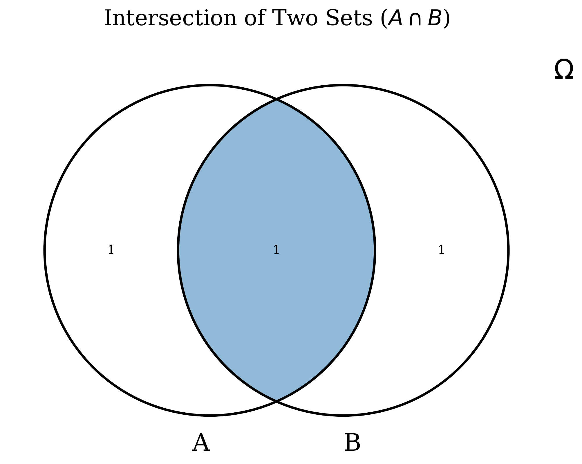
The intersection of sets $A$ and $B$ is the set containing all elements that are common to both $A$ and $B$ [3].

A \cap B = \{x \mid x \in A \text{ and } x \in B\}

Example 5: Intersection

If $A = \{1, 2, 3\}$ and $B = \{3, 4, 5\}$, then $A \cap B = \{3\}$.

If $C = \{1, 2\}$ and $D = \{3, 4\}$, then $C \cap D = \emptyset$.

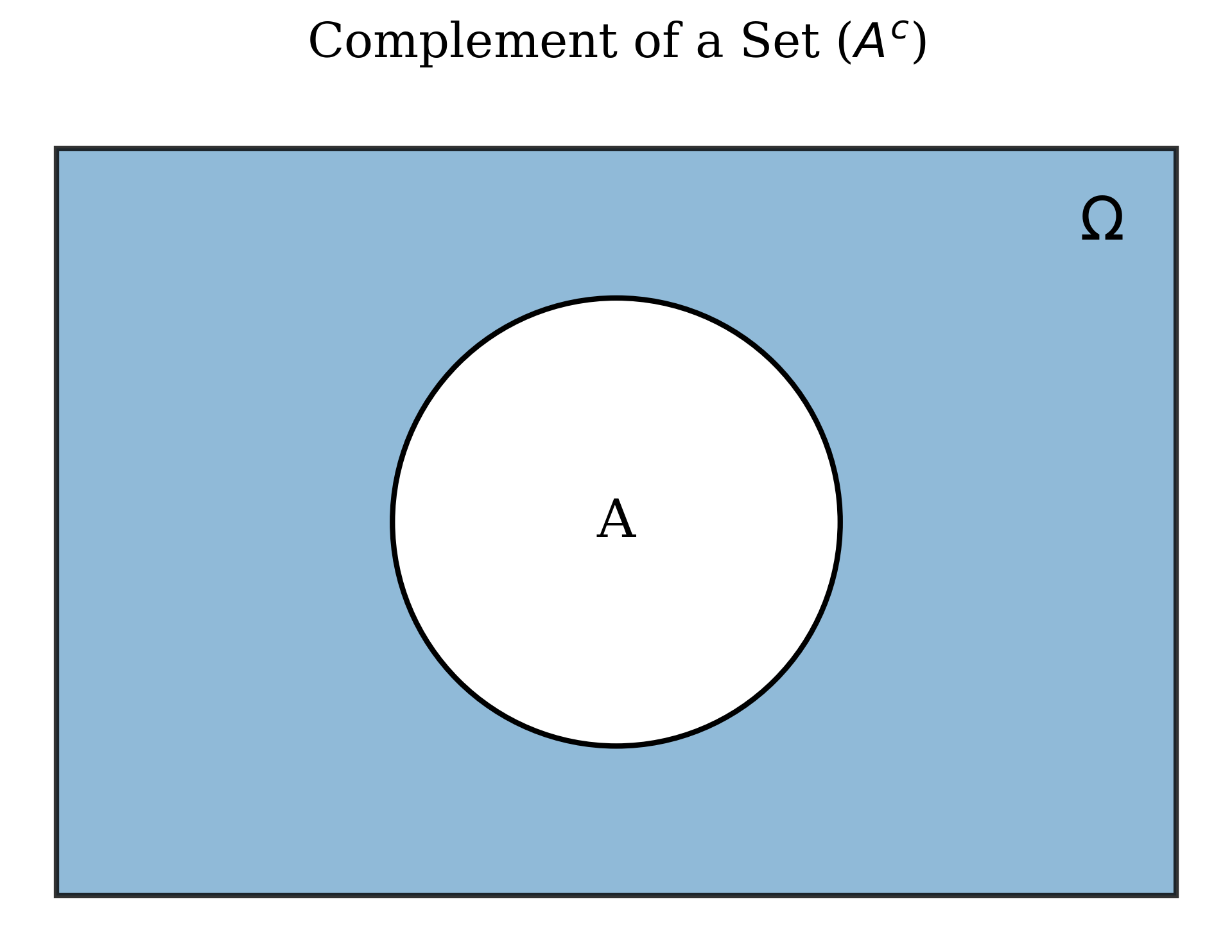
Venn Diagram for Intersection $A \cap B$

Definition: Complement ($A^c$ or $\bar{A}$)

Relative to a universal set $\Omega$, the complement of $A$ is the set of all elements in $\Omega$ that are not in $A$ [1][3].

A^c = \{x \mid x \in \Omega \text{ and } x \notin A\}

Definition: Set Difference ($A \setminus B$)

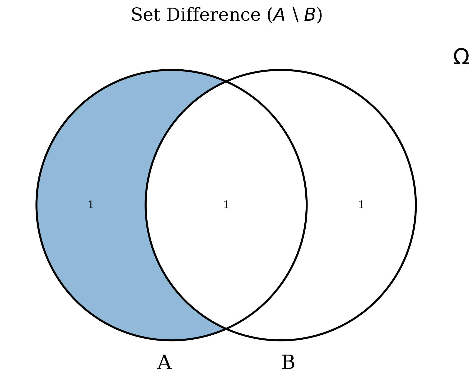
The difference of sets $A$ and $B$ is the set containing all elements that are in $A$ but not in $B$ [1][4].

A \setminus B = \{x \mid x \in A \text{ and } x \notin B\}

Note that $A \setminus B = A \cap B^c$.

Venn Diagram for Set Difference $A \setminus B$

Disjoint Sets and Partitions

Definition: Disjoint Sets

Two sets $A$ and $B$ are disjoint (or mutually exclusive) if they have no elements in common, i.e., $A \cap B = \emptyset$ [1][4].

Definition: Partition

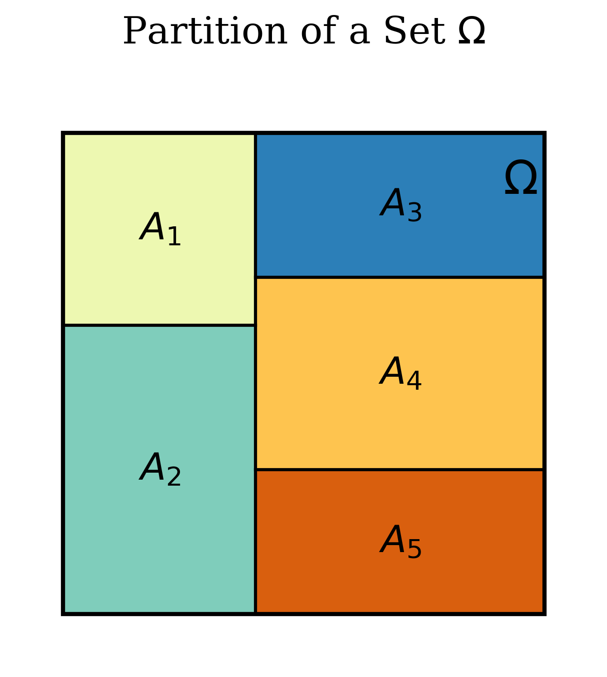
A collection of non-empty sets $\{A_1, \ldots, A_n\}$ forms a partition of a set $\Omega$ if [1][4]:

The sets are pairwise disjoint: $A_i \cap A_j = \emptyset$ for all $i \ne j$.
The sets are collectively exhaustive: $\displaystyle \bigcup_{i=1}^n A_i = \Omega$.

Set Algebra Properties

These properties are essential for manipulating sets.

Commutative Laws: $A \cup B = B \cup A$; $A \cap B = B \cap A$ [1][4].
Associative Laws: $A \cup (B \cup C) = (A \cup B) \cup C$; $A \cap (B \cap C) = (A \cap B) \cap C$ [1][4].
Distributive Laws: $A \cap (B \cup C) = (A \cap B) \cup (A \cap C)$; $A \cup (B \cap C) = (A \cup B) \cap (A \cup C)$ [1][4].
De Morgan's Laws: $(A \cup B)^c = A^c \cap B^c$; $(A \cap B)^c = A^c \cup B^c$ [1][4].

Cardinality and Countability

Understanding the "size" of sets, especially infinite sets, is important for defining sample spaces.

Equicardinality and Bijective Functions

Definition: Equicardinal Sets

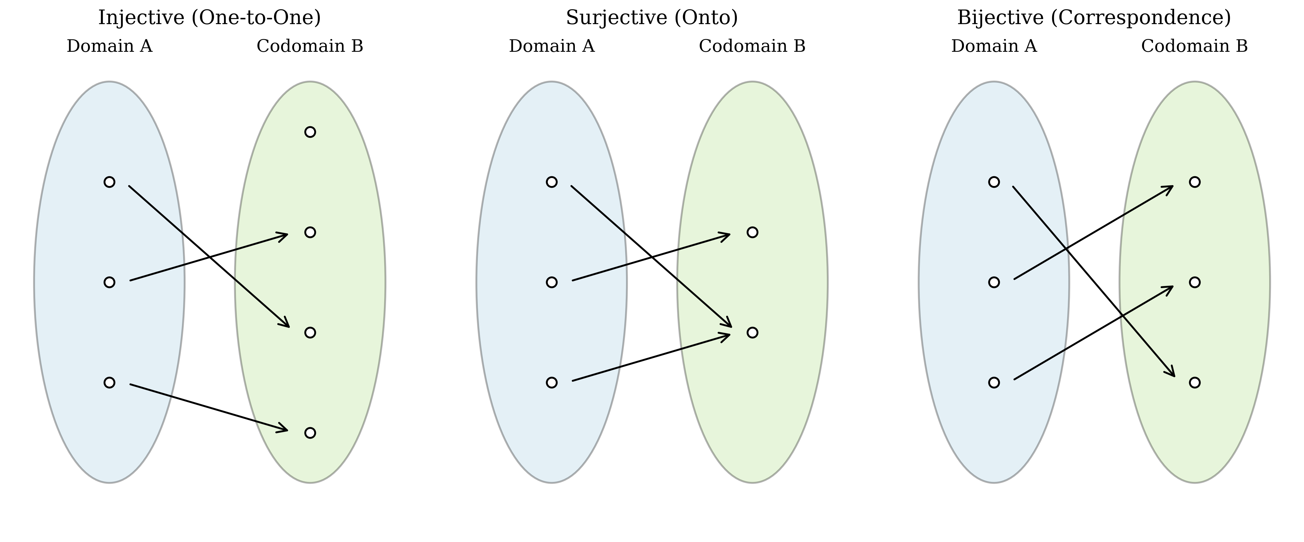
Two sets $A$ and $B$ are equicardinal (have the same cardinality) if there exists a bijective function $f: A \to B$ between them [1][4].

Definition: Bijective Function

A function $f: A \to B$ is bijective (or a one-to-one correspondence) if it is both:

Injective (One-to-One): For every $a_1, a_2 \in A$, if $f(a_1) = f(a_2)$, then $a_1 = a_2$. (Distinct inputs map to distinct outputs) [1].
Surjective (Onto): For every $b \in B$, there exists at least one $a \in A$ such that $f(a) = b$. (Every element in the codomain is mapped to) [1].

Function Types — Illustrations of injective, surjective, and bijective functions

Types of Sets by Cardinality

Finite Set: A set that is equicardinal with $\{1, 2, \ldots, n\}$ for some non-negative integer $n$. Its cardinality is $n$ [1].
Infinite Set: A set that is not finite [1].
- Countably Infinite Set: An infinite set that is equicardinal with the set of natural numbers $\mathbb{N} = \{1,2,3,\ldots\}$ [1][4].
- Uncountable Set: An infinite set that is not countably infinite [1][4].

Definition: Countable Set

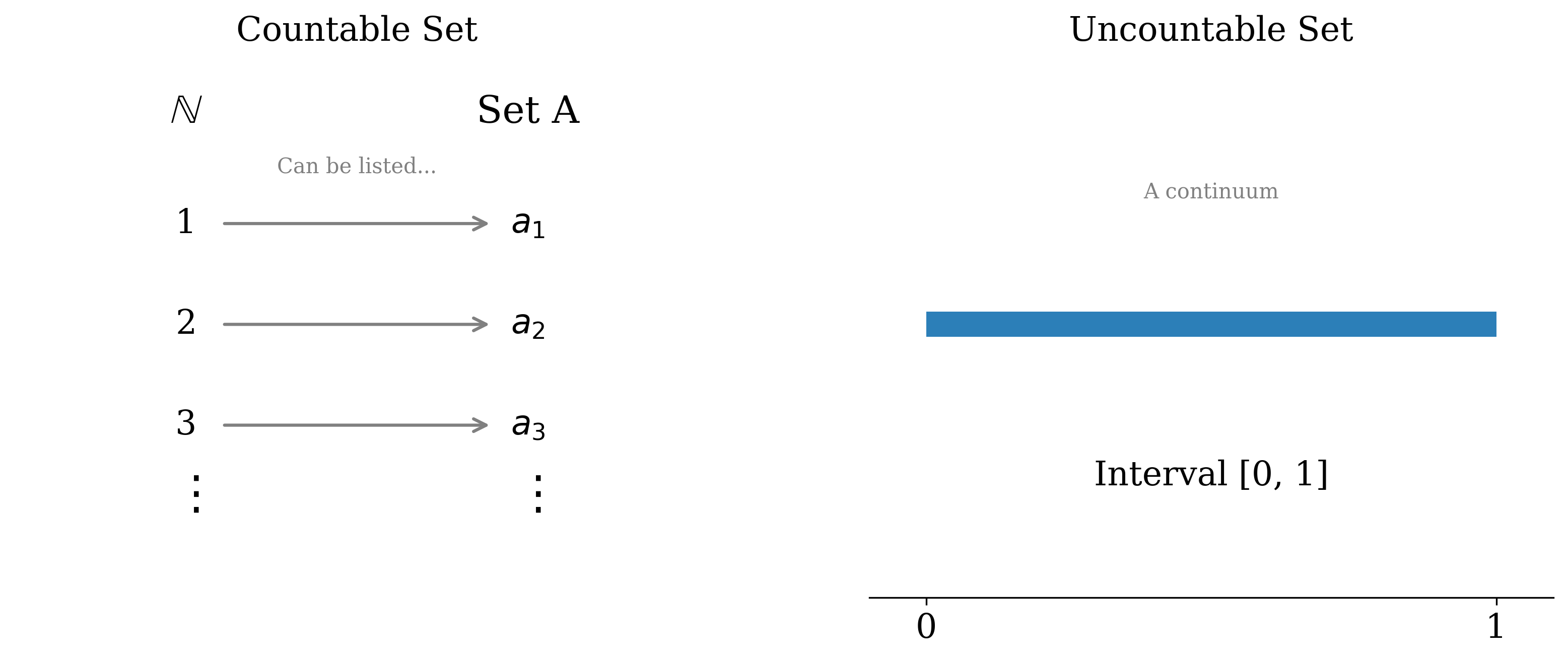
A set is countable if it is either finite or countably infinite [4].

Example 6: Countable and Uncountable Sets

$\mathbb{N}$ (natural numbers), $\mathbb{Z}$ (integers), $\mathbb{Q}$ (rational numbers) are countable [1][4].
$\mathbb{R}$ (real numbers), intervals like $[0,1]$ or $(0,1)$ are uncountable [1][4].

Remark

Every countably infinite set can be listed as a sequence.

Countability Visualization — Visualization of countable and uncountable sets

The Probability Space $(\Omega, \mathcal{F}, \mathbb{P})$

Probability theory provides a mathematical framework for modeling experiments with random outcomes. This framework is the probability space, a triplet $(\Omega, \mathcal{F}, \mathbb{P})$ [2][4].

Component 1: The Sample Space ($\Omega$)

Definition: Sample Space

The Sample Space ($\Omega$) is the set of all possible outcomes of a random experiment [3][4]. Each outcome $w$ is an element of $\Omega$ ($w \in \Omega$). A sample space must be exhaustive (includes all possibilities) and its elements must be mutually exclusive (distinct outcomes) [4].

Example 7: Sample Spaces

Experiment: Flip a coin. $\Omega = \{H, T\}$ [3].
Experiment: Roll a die. $\Omega = \{1, 2, 3, 4, 5, 6\}$ [3].
Experiment: Measure lifetime of a device. $\Omega = [0, \infty) = \{t \mid t \ge 0\}$ [3].

Component 2: The Event Space ($\mathcal{F}$)

Definition: Event

An Event ($A$) is a subset of the sample space ($A \subseteq \Omega$) [3][4]. An event is said to occur if the outcome of the experiment is an element of that event.

Example 8: Events

Experiment: Roll a die, $\Omega = \{1, 2, 3, 4, 5, 6\}$.

Event $A$: "An even number is rolled." $A = \{2, 4, 6\}$.
Event $B$: "A number less than 3 is rolled." $B = \{1, 2\}$.
Event $C$: "The number 5 is rolled." $C = \{5\}$.

Definition: Event Space ($\sigma$-field)

The Event Space ($\mathcal{F}$) is a collection of subsets of $\Omega$ (i.e., a set of events) that satisfies the properties of a $\sigma$-field (or $\sigma$-algebra). This ensures that we can consistently assign probabilities and perform operations like complements and unions [4].

A collection $\mathcal{F}$ of subsets of $\Omega$ is a $\sigma$-field if:

$\Omega \in \mathcal{F}$ (The sample space itself is an event).
If $A \in \mathcal{F}$, then $A^c \in \mathcal{F}$ (Closed under complementation).
If $A_1, A_2, \ldots \in \mathcal{F}$ (a countable sequence), then $\displaystyle \bigcup_{i=1}^{\infty} A_i \in \mathcal{F}$ (Closed under countable unions).

Remark

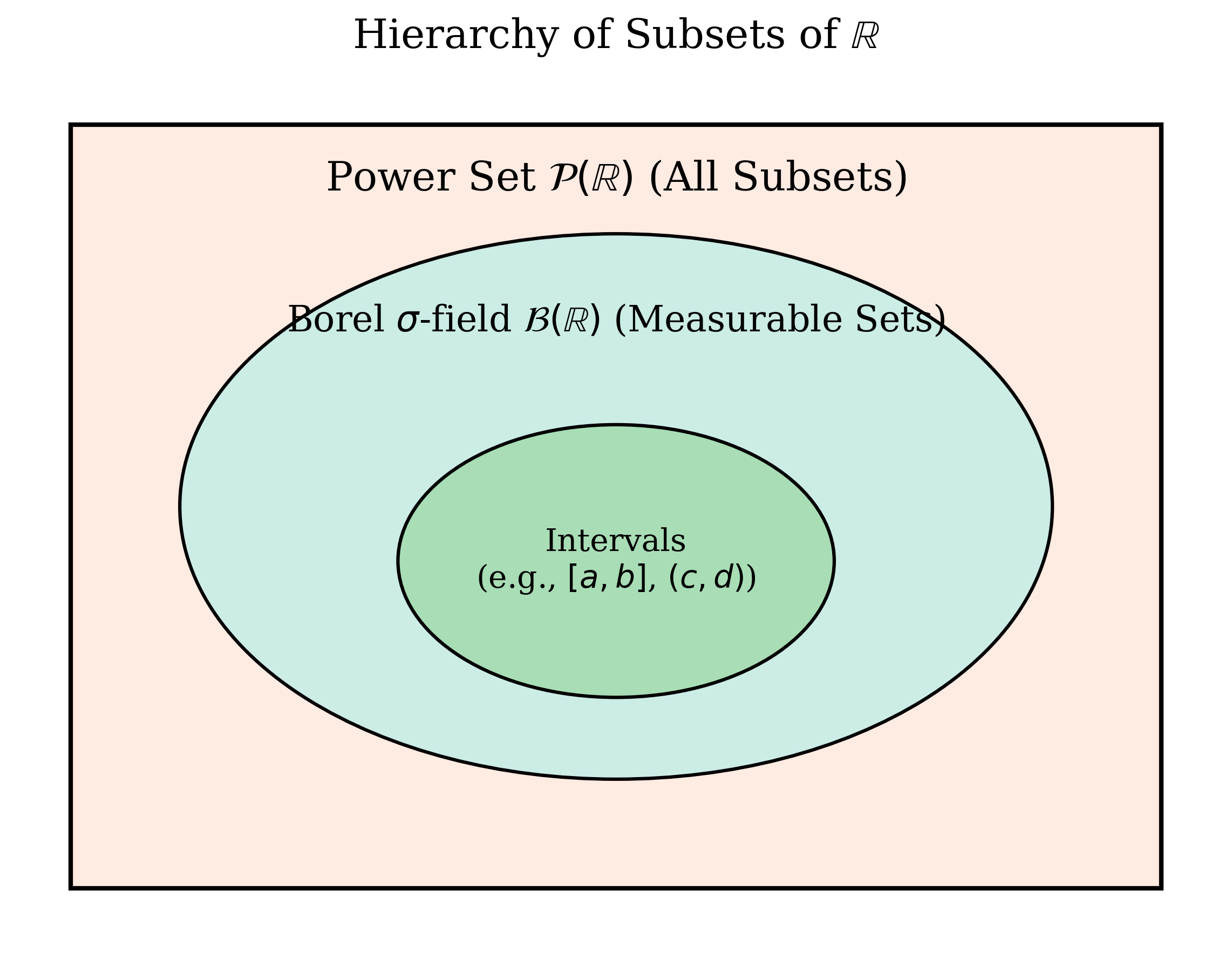
For discrete sample spaces, $\mathcal{F}$ is usually the power set $P(\Omega)$ (the set of all subsets) [1][4]. For continuous spaces like $\mathbb{R}$, $\mathcal{F}$ is the Borel $\sigma$-field $\mathcal{B}(\mathbb{R})$, generated by intervals [2][4].

Component 3: The Probability Law ($\mathbb{P}$)

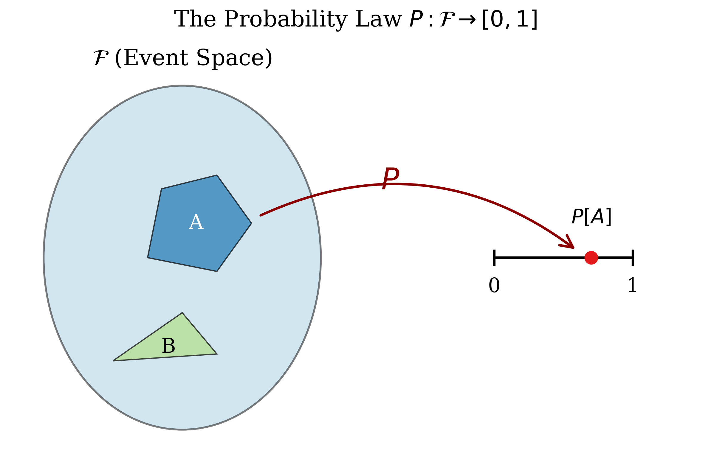
Definition: Probability Law/Measure

The Probability Law or Probability Measure $\mathbb{P}$ is a function that assigns a real number $\mathbb{P}[A]$ to each event $A \in \mathcal{F}$, satisfying the Axioms of Probability [2][4].

\mathbb{P}: \mathcal{F} \rightarrow [0, 1]

It quantifies the likelihood of each measurable event in $\mathcal{F}$, serving as a measure of its relative size within the sample space [4].

Probability Law Mapping — The Probability Law $\mathbb{P}$ maps events from $\mathcal{F}$ to values in $[0, 1]$

Measurable Sets and the Need for a $\sigma$-Field

Not every subset of a sample space can be consistently assigned a probability. To avoid contradictions, probability is defined only on a specific collection of subsets $\mathcal{F}$ called a $\sigma$-field.

The sets in $\mathcal{F}$ are called measurable sets. A probability measure $\mathbb{P}$ assigns values only to these measurable events, not to arbitrary subsets [4].

Remark

In continuous sample spaces such as $\mathbb{R}$, the event space is usually the Borel $\sigma$-field $\mathcal{B}(\mathbb{R})$, which contains intervals and any set formed from them using countable unions, intersections, and complements.

Example 9: Measurable Sets

Every interval in $\mathbb{R}$ such as $(0,1)$ or $[2,\infty)$ is measurable. However, there exist subsets of $\mathbb{R}$ that are not measurable, and probability cannot be meaningfully assigned to them.

Measurable Sets Illustration — Visualization of measurable sets within a $\sigma$-field

Intuitively, probability measures the likelihood of measurable events. A $\sigma$-field ensures that this measurement behaves consistently.

The Axioms of Probability

Any function $\mathbb{P}: \mathcal{F} \to [0, 1]$ must satisfy the following three axioms to be considered a valid probability measure [3][4].

Axiom I: Non-negativity

For any event $A \in \mathcal{F}$,

\mathbb{P}[A] \ge 0

Axiom II: Normalization

The probability assigned to the entire sample space is 1.

\mathbb{P}[\Omega] = 1

Axiom III: Countable Additivity

For any countable sequence of pairwise disjoint events $\{A_1, A_2, \ldots\} \subseteq \mathcal{F}$ (i.e., $A_i \cap A_j = \emptyset$ for all $i \ne j$), the probability of their union is the sum of their individual probabilities.

\mathbb{P}\left[\bigcup_{i=1}^{\infty} A_i\right] = \sum_{i=1}^{\infty} \mathbb{P}[A_i]

Remark

Axiom III implies finite additivity: For any finite collection of pairwise disjoint events $A_1, \ldots, A_n$,

\mathbb{P}\left[\bigcup_{i=1}^{n} A_i\right] = \sum_{i=1}^{n} \mathbb{P}[A_i]

In particular, for two disjoint events $A$ and $B$, $\mathbb{P}[A \cup B] = \mathbb{P}[A] + \mathbb{P}[B]$ [4].

Corollaries from the Axioms

These fundamental properties are direct consequences of the axioms.

Corollary 1: Probability of the Complement

For any event $A$, $\mathbb{P}[A^c] = 1 - \mathbb{P}[A]$ [2][3][4].

Proof:

Since $A$ and $A^c$ form a partition of $\Omega$ (they are disjoint and $A \cup A^c = \Omega$), Axioms II and III (finite additivity) give:

1 = \mathbb{P}[\Omega] = \mathbb{P}[A \cup A^c] = \mathbb{P}[A] + \mathbb{P}[A^c]

Rearranging yields the result.

Corollary 2: Probability of the Empty Set

$\mathbb{P}[\emptyset] = 0$ [2][3][4].

Proof:

Since $\emptyset = \Omega^c$, apply Corollary 1: $\mathbb{P}[\emptyset] = \mathbb{P}[\Omega^c] = 1 - \mathbb{P}[\Omega] = 1 - 1 = 0$.

Corollary 3: Monotonicity

If $A \subseteq B$, then $\mathbb{P}[A] \le \mathbb{P}[B]$ [4].

Proof:

We can write $B = A \cup (B \setminus A)$. The sets $A$ and $B \setminus A$ are disjoint. By Axiom III, $\mathbb{P}[B] = \mathbb{P}[A] + \mathbb{P}[B \setminus A]$. Since $\mathbb{P}[B \setminus A] \ge 0$ by Axiom I, it follows that $\mathbb{P}[B] \ge \mathbb{P}[A]$.

Corollary 4: Inclusion-Exclusion Principle (for 2 events)

For any two events $A$ and $B$:

\mathbb{P}[A \cup B] = \mathbb{P}[A] + \mathbb{P}[B] - \mathbb{P}[A \cap B]

[2][3][4]

Proof:

We can write $A \cup B$ as the union of three disjoint sets: $(A \setminus B)$, $(B \setminus A)$, and $(A \cap B)$.

Thus, $\mathbb{P}[A \cup B] = \mathbb{P}[A \setminus B] + \mathbb{P}[B \setminus A] + \mathbb{P}[A \cap B]$.

Also, $A = (A \setminus B) \cup (A \cap B)$ (disjoint union), so $\mathbb{P}[A] = \mathbb{P}[A \setminus B] + \mathbb{P}[A \cap B]$, which implies $\mathbb{P}[A \setminus B] = \mathbb{P}[A] - \mathbb{P}[A \cap B]$.

Similarly, $\mathbb{P}[B \setminus A] = \mathbb{P}[B] - \mathbb{P}[A \cap B]$.

Substituting these into the first equation gives:

\mathbb{P}[A \cup B] = (\mathbb{P}[A] - \mathbb{P}[A \cap B]) + (\mathbb{P}[B] - \mathbb{P}[A \cap B]) + \mathbb{P}[A \cap B]

which simplifies to $\mathbb{P}[A \cup B] = \mathbb{P}[A] + \mathbb{P}[B] - \mathbb{P}[A \cap B]$.

Conditional Probability

Conditional probability allows us to update the probability of an event based on the knowledge that another event has occurred.

Definition

Definition: Conditional Probability

Given two events $A$ and $B$, with $\mathbb{P}[B] > 0$, the conditional probability of $A$ given $B$ is defined as:

\mathbb{P}[A \mid B] = \frac{\mathbb{P}[A \cap B]}{\mathbb{P}[B]}

[2]

Remark

Intuitively, knowing that $B$ has occurred restricts the relevant sample space to just the outcomes within $B$. $\mathbb{P}[A \mid B]$ measures the proportion of the probability mass within $B$ that also corresponds to outcomes in $A$.

Conditional Probability as a Valid Probability Measure

For a fixed event $B$ with $\mathbb{P}[B] > 0$, the function $P_B(\cdot) = \mathbb{P}[\cdot \mid B]$ defines a new, valid probability measure on the original sample space $\Omega$ and event space $\mathcal{F}$. It satisfies the three axioms [2].

Proof: Verifying the axioms for $P_B(\cdot)$

Non-negativity: For any event $A$, $\mathbb{P}[A \cap B] \ge 0$ (Axiom I for $\mathbb{P}$) and $\mathbb{P}[B] > 0$. Therefore, $P_B(A) = \dfrac{\mathbb{P}[A \cap B]}{\mathbb{P}[B]} \ge 0$.
Normalization: We need to show $P_B(\Omega) = 1$. $P_B(\Omega) = \mathbb{P}[\Omega \mid B] = \dfrac{\mathbb{P}[\Omega \cap B]}{\mathbb{P}[B]}$. Since $B \subseteq \Omega$, $\Omega \cap B = B$. Thus, $P_B(\Omega) = \dfrac{\mathbb{P}[B]}{\mathbb{P}[B]} = 1$.
Countable Additivity: Let $A_1, A_2, \ldots$ be a sequence of pairwise disjoint events. We need to show $P_B(\bigcup A_i) = \sum P_B(A_i)$. $\begin{align} P_B\left(\bigcup_{i=1}^{\infty} A_i\right) &= \mathbb{P}\left[\bigcup_{i=1}^{\infty} A_i \;\middle|\; B\right] \\ &= \frac{\mathbb{P}\left[\left(\bigcup_{i=1}^{\infty} A_i\right) \cap B\right]}{\mathbb{P}[B]} \\ &= \frac{\mathbb{P}\left[\bigcup_{i=1}^{\infty} (A_i \cap B)\right]}{\mathbb{P}[B]} \end{align}$
Since $A_i$ are disjoint, the events $(A_i \cap B)$ are also disjoint. Applying Axiom III for $\mathbb{P}$:
$\begin{align} P_B\left(\bigcup_{i=1}^{\infty} A_i\right) &= \frac{\sum_{i=1}^{\infty} \mathbb{P}[A_i \cap B]}{\mathbb{P}[B]} \\ &= \sum_{i=1}^{\infty} \frac{\mathbb{P}[A_i \cap B]}{\mathbb{P}[B]} \\ &= \sum_{i=1}^{\infty} \mathbb{P}[A_i \mid B] = \sum_{i=1}^{\infty} P_B(A_i) \end{align}$

Thus, $P_B(\cdot)$ is a valid probability measure.

Back to Notebook Index

Set Theory and Probability I

Set Theory

Sets and Elements

Describing Sets

Fundamental Set Concepts

Set Operations

Disjoint Sets and Partitions

Set Algebra Properties

Cardinality and Countability

Equicardinality and Bijective Functions

Types of Sets by Cardinality

The Probability Space \((\Omega, \mathcal{F}, \mathbb{P})\)

Component 1: The Sample Space (\(\Omega\))

Component 2: The Event Space (\(\mathcal{F}\))

Component 3: The Probability Law (\(\mathbb{P}\))

Measurable Sets and the Need for a \(\sigma\)-Field

The Axioms of Probability

Corollaries from the Axioms

Conditional Probability

Definition

Conditional Probability as a Valid Probability Measure