Mathematical Background Review

October 24, 2025 Computer Science Mathematics & Probability

This document reviews foundational mathematical concepts frequently used in computer science, data science, and engineering. Data science is fundamentally about making decisions under uncertainty, and probability is the mathematical tool for modeling, analyzing, and predicting random events. This review covers topics including functions, polynomials, infinite series (geometric, Taylor), combinatorics (permutations, combinations, binomial theorem), and integration techniques, all of which are essential for this analysis [1]. This document combines notes originally prepared by Md Shahriar Karim [2] with theoretical background from [1].

Functions: Inverses and Properties

Inverse Functions

A function $f$ is invertible if and only if it is a bijection, meaning it is both:

One-to-one (Injective): Each element in the range is mapped to by at most one element in the domain.
Onto (Surjective): Each element in the range is mapped to by at least one element in the domain.

When we invert a function, the range of the original function $f$ becomes the domain for the inverse function $f -1$ .

Example 1: Finding an Inverse

Find the inverse of $f(x) = \dfrac{2}{e^x + 1}$.

Let $y = f(x)$. We solve for $x$:

\begin{align} y &= \frac{2}{e^x + 1} \\ y(e^x + 1) &= 2 \\ ye^x + y &= 2 \\ ye^x &= 2 - y \\ e^x &= \frac{2-y}{y} \\ x &= \ln\left(\frac{2-y}{y}\right) = \ln\left(\frac{2}{y} - 1\right) \end{align}

Therefore, the inverse function is $f^{-1}(y) = \ln\left(\dfrac{2}{y} - 1\right)$. Swapping variables to use $x$, we get:

f^{-1}(x) = \ln\left(\frac{2}{x} - 1\right)

Checking for One-to-One (Injective)

A function is one-to-one if $f(x 1) = f(x 2)$ implies $x 1 = x 2$ .

Example 2: Testing One-to-One Property

Is $f(x) = \dfrac{x+5}{x-6}$ one-to-one?

Set $f(x_1) = f(x_2)$:

\begin{align} \frac{x_1+5}{x_1-6} &= \frac{x_2+5}{x_2-6} \\ (x_1+5)(x_2-6) &= (x_2+5)(x_1-6) \\ x_1x_2 - 6x_1 + 5x_2 - 30 &= x_1x_2 + 5x_1 - 6x_2 - 30 \\ -6x_1 + 5x_2 &= 5x_1 - 6x_2 \\ 11x_2 &= 11x_1 \Rightarrow x_1 = x_2 \end{align}

Yes, the function is one-to-one.

A strictly increasing or strictly decreasing function (where $f'(x) > 0$ or $f'(x) < 0$ for all $x$ in the domain) is always one-to-one.

Example 3: One-to-One via Derivative

Is $f(x) = xe^{x^4}$ one-to-one for $x \in \mathbb{R}$?

We check its derivative, $f'(x)$:

\begin{align} f'(x) &= (1) \cdot e^{x^4} + x \cdot (e^{x^4} \cdot 4x^3) \\ &= e^{x^4} + 4x^4 e^{x^4} \\ &= e^{x^4}(1 + 4x^4) \end{align}

Since $e^{x^4}$ is always positive and $(1 + 4x^4)$ is always positive for any real $x$, $f'(x)$ is always positive. Because $f'(x) > 0$ for all $x$, the function is strictly increasing, and therefore it is one-to-one.

Polynomials

A polynomial of degree $n$ is a function of the form:

f(x) = a n x n + a n-1 x n-1 + \dots + a 1 x + a 0

The degree is the highest power of $x$ with a non-zero coefficient.

Roots and Multiplicity

The roots of a polynomial are the values of $x$ for which $f(x) = 0$ .

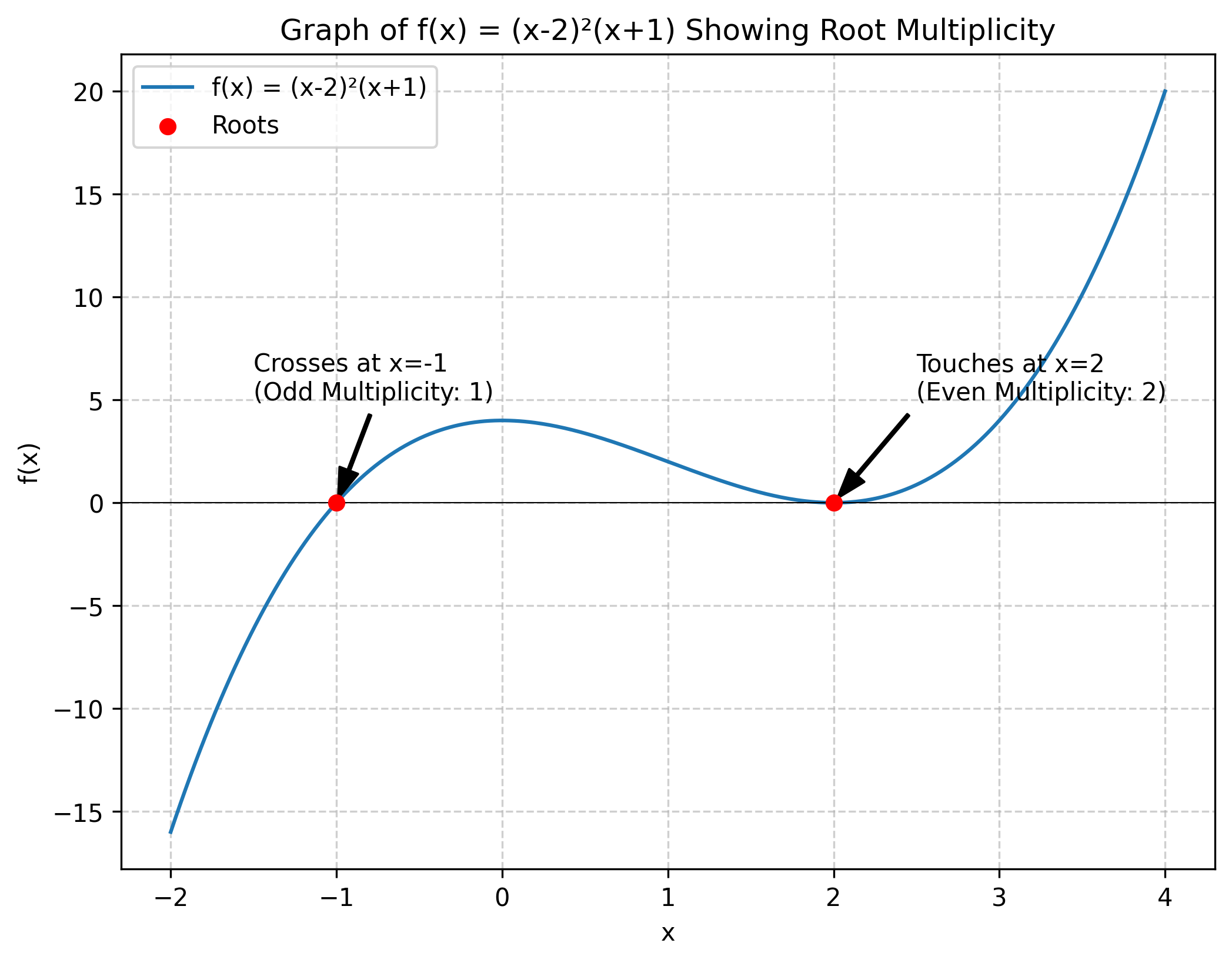
The multiplicity of a root is the number of times it appears as a factor. For example, in $f(x) = (x-2) 3 (x+4) 1$ , the root $x=2$ has a multiplicity of 3, and the root $x=-4$ has a multiplicity of 1.

The multiplicity of a root provides graphical information:

Even multiplicity: The graph touches the x-axis at the root and turns around.
Odd multiplicity: The graph crosses the x-axis at the root.

Example 4: Sketching with Multiplicity

Sketch $f(x) = (x-2)^2(x+1)$.

Roots are $x=2$ (multiplicity 2, even) and $x=-1$ (multiplicity 1, odd).
The graph will touch the x-axis at $x=2$.
The graph will cross the x-axis at $x=-1$.

Infinite Series and Approximations

Infinite series are used frequently in probability, such as when evaluating the expectation and variance of random variables [1].

Geometric Series

A geometric series is a sequence where each term after the first is found by multiplying the previous one by a fixed, non-zero number called the common ratio, $r$ .

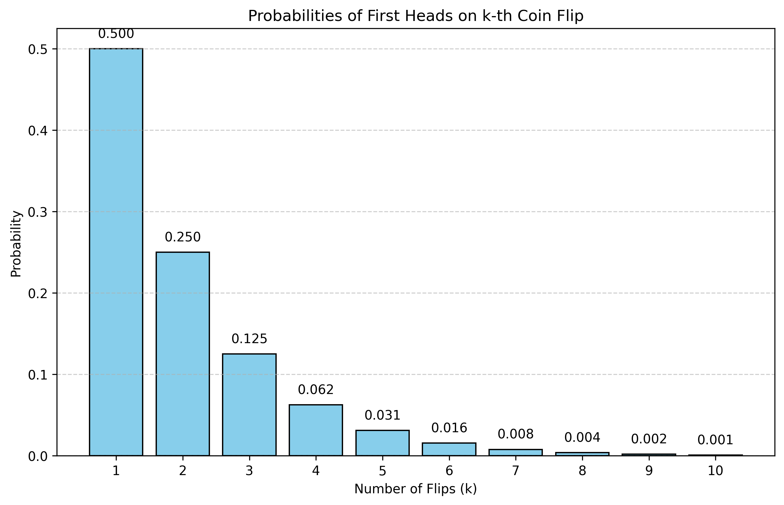
Example 5: Motivating Example - Coin Flip

Imagine you flip a fair coin until you get a head [1].

P(1 flip: H) = $\frac{1}{2}$
P(2 flips: TH) = $\frac{1}{2} \times \frac{1}{2} = \frac{1}{4}$
P(3 flips: TTH) = $\frac{1}{2} \times \frac{1}{2} \times \frac{1}{2} = \frac{1}{8}$

The sequence of probabilities is $\left\{\frac{1}{2}, \frac{1}{4}, \frac{1}{8}, \ldots\right\}$, a geometric sequence with first term $a = \frac{1}{2}$ and common ratio $r = \frac{1}{2}$.

Theorem 1: Sum of a Finite Geometric Series

The sum of the first $n+1$ terms of a geometric series (starting from $k=0$) with first term $a$ and common ratio $r$ is [1]:

S_n = \sum_{k=0}^{n} ar^k = a + ar + ar^2 + \cdots + ar^n = \frac{a(1-r^{n+1})}{1-r}, \quad r \neq 1

For the simple case $a=1$: $\displaystyle \sum_{k=0}^{n} r^k = \frac{1-r^{n+1}}{1-r}$.

Corollary 1: Sum of an Infinite Geometric Series

If $0 < |r| < 1$, the sum of an infinite geometric series converges to [1]:

S_{\infty} = \sum_{k=0}^{\infty} ar^k = a + ar + ar^2 + \cdots = \frac{a}{1-r}

For the simple case $a=1$: $\displaystyle \sum_{k=0}^{\infty} r^k = \frac{1}{1-r}$. This works because as $n \to \infty$, the term $r^{n+1}$ approaches 0.

Example 6: Computing an Infinite Geometric Series

Compute $\displaystyle \sum_{k=2}^{\infty} \frac{1}{2^k}$.

This series is $\frac{1}{4} + \frac{1}{8} + \frac{1}{16} + \cdots$

The first term is $a = \frac{1}{4}$ and the common ratio is $r = \frac{1}{2}$. Since $|r|<1$, the series converges.

Using the infinite sum formula:

S_{\infty} = \frac{a}{1-r} = \frac{\frac{1}{4}}{1 - \frac{1}{2}} = \frac{\frac{1}{4}}{\frac{1}{2}} = \frac{1}{4} \cdot \frac{2}{1} = \frac{1}{2}

Corollary 2: Derivative of Geometric Series

By taking the derivative of the infinite series formula $\displaystyle \sum_{k=0}^{\infty} r^k = \frac{1}{1-r}$ with respect to $r$, we get a useful identity for $0 < |r| < 1$ [1]:

\begin{align} \frac{d}{dr} \sum_{k=0}^{\infty} r^k &= \frac{d}{dr} \left(\frac{1}{1-r}\right) \\ \sum_{k=1}^{\infty} kr^{k-1} &= 1 + 2r + 3r^2 + \cdots = \frac{1}{(1-r)^2} \end{align}

Example 7: Using the Derivative Formula

Compute $\displaystyle \sum_{k=1}^{\infty} k \cdot \frac{2}{3^k}$.

We can manipulate this to match the corollary:

\begin{align} \sum_{k=1}^{\infty} k \cdot \frac{2}{3^k} &= 2 \sum_{k=1}^{\infty} k \cdot \left(\frac{1}{3}\right)^k \\ &= 2 \cdot \frac{1}{3} \sum_{k=1}^{\infty} k \cdot \left(\frac{1}{3}\right)^{k-1} \end{align}

Now apply the formula with $r = \frac{1}{3}$:

= \frac{2}{3} \cdot \frac{1}{\left(1 - \frac{1}{3}\right)^2} = \frac{2}{3} \cdot \frac{1}{\left(\frac{2}{3}\right)^2} = \frac{2}{3} \cdot \frac{1}{\frac{4}{9}} = \frac{2}{3} \cdot \frac{9}{4} = \frac{3}{2}

Taylor and Maclaurin Series

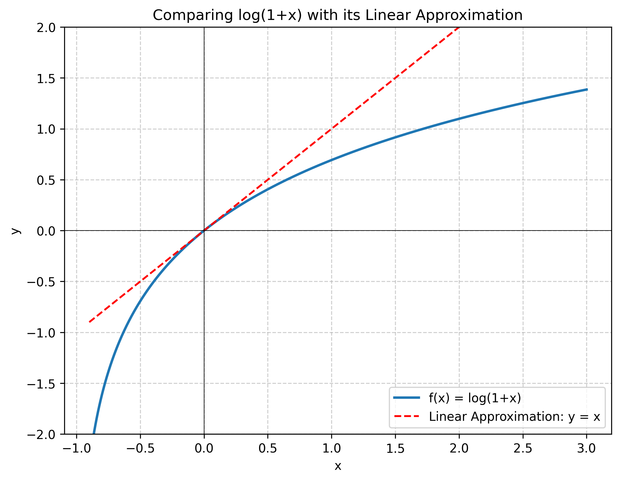
Taylor approximation is a powerful tool for approximating complex, non-linear functions (like $log(1+x)$ ) with simpler polynomials. This is especially useful for analysis when $x$ is close to a certain point $a$ , e.g., $x ≪ 1$ [1].

Definition: Taylor Approximation

The Taylor approximation of an infinitely differentiable function $f(x)$ at a point $x=a$ is [1]:

f(x) = \sum_{n=0}^{\infty} \frac{f^{(n)}(a)}{n!} (x-a)^n = f(a) + f'(a)(x-a) + \frac{f''(a)}{2!} (x-a)^2 + \cdots

When $a=0$, this is called a Maclaurin Series.

Example 8: $f(x) = e^x$ at $a=0$

All derivatives $f^{(n)}(x)$ are $e^x$, so $f^{(n)}(0) = e^0 = 1$ for all $n$.

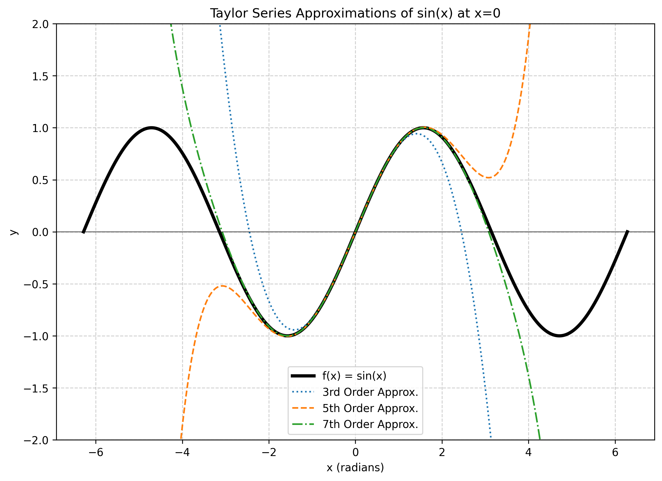
e^x = \sum_{n=0}^{\infty} \frac{1}{n!} (x-0)^n = 1 + x + \frac{x^2}{2!} + \frac{x^3}{3!} + \cdots

Example 9: $f(x) = \sin x$ at $a=0$

The derivatives at $x=0$ follow a pattern: $f(0)=0$, $f'(0)=1$, $f''(0)=0$, $f'''(0)=-1$, etc. Plugging these into the formula, all the even-powered terms go to zero:

\begin{align} \sin x &= 0 + \frac{1}{1!}x + 0 + \frac{-1}{3!}x^3 + 0 + \frac{1}{5!}x^5 + \cdots \\ \sin x &= x - \frac{x^3}{3!} + \frac{x^5}{5!} - \frac{x^7}{7!} + \cdots \end{align}

As you include more terms, the approximation becomes more accurate over a wider range.

Combinatorics

Combinatorics is the field of mathematics concerned with counting configurations of discrete events.

Example 10: Motivating Example - Birthday Paradox

In a room of $k$ people, what is the probability that at least one pair shares a birthday [1]?

It's easier to calculate the complement: the probability that no one shares a birthday (assuming 365 days).

Person 1: $\frac{365}{365}$ (can have any birthday)
Person 2: $\frac{364}{365}$ (must be different from person 1)
Person 3: $\frac{363}{365}$ (must be different from 1 and 2)
...
Person k: $\frac{365 - k + 1}{365}$

The probability of all $k$ people having different birthdays is:

P(\text{all different}) = \frac{365 \times 364 \times \cdots \times (365-k+1)}{365^k} = \frac{365!}{(365-k)!} \cdot \frac{1}{365^k}

For $k=50$ people, $P(\text{all different}) \approx 0.03$. So, the probability of at least one match is $P(\text{match}) = 1 - 0.03 = 0.97$, or 97%!

Permutation

A permutation is an ordered arrangement of $k$ items selected from a set of $n$ distinct items without replacement.

Theorem 2: Number of Permutations

The number of ways to choose $k$ ordered items from $n$ is [1]:

P(n, k) = n(n-1)(n-2)\cdots(n-k+1) = \frac{n!}{(n-k)!}

Example 11: Awarding Prizes

How many ways to award 1st, 2nd, and 3rd prize (ordered) from 100 contestants?

P(100, 3) = \frac{100!}{(100-3)!} = \frac{100!}{97!} = 100 \times 99 \times 98 = 970{,}200

Example 12: String Permutations

How many permutations of the letters ABCDEFG contain:

the string BCD?
Treat (BCD) as a single block. We are permuting (BCD), A, E, F, G. These are 5 distinct items. So, the total permutations is $5! = 120$ .
the strings BA and GF?
Treat (BA) and (GF) as single blocks. We are permuting (BA), (GF), C, D, E. These are 5 distinct items. So, the total permutations is $5! = 120$ .
the strings ABC and CDE?
This implies the string must be (ABCDE). We are permuting (ABCDE), F, G. These are 3 distinct items. So, the total permutations is $3! = 6$ .
the strings CBA and BED?
This is impossible, as the letter 'B' must be in two different positions simultaneously. The number of permutations is 0.

Combination

A combination is an unordered selection of $k$ items from a set of $n$ distinct items without replacement. The order of selection does not matter.

Theorem 3: Number of Combinations

This is also called "n choose k" or the binomial coefficient [1].

C(n, k) = \binom{n}{k} = \frac{P(n, k)}{k!} = \frac{n!}{k!(n-k)!}

We divide the number of permutations by $k!$ because there are $k!$ ways to order the $k$ chosen items, and in a combination, all those orderings are counted as one.

Example 13: Poker Hands

How many 5-card poker hands (unordered) can be dealt from a standard 52-card deck?

C(52, 5) = \binom{52}{5} = \frac{52!}{5!(52-5)!} = \frac{52!}{5! \cdot 47!} = 2{,}598{,}960

Example 14: Selecting a Crew

How many ways to select a 6-person crew (unordered) from 30 astronauts?

C(30, 6) = \binom{30}{6} = \frac{30!}{6!(30-6)!} = \frac{30!}{6! \cdot 24!} = 593{,}775

The Binomial Theorem

The binomial theorem uses combinations (binomial coefficients) to expand a binomial raised to a power.

Theorem 4: Binomial Theorem

For any real numbers $a$ and $b$ and integer $n \geq 0$ [1]:

(a+b)^n = \sum_{k=0}^{n} \binom{n}{k} a^{n-k}b^k

Example 15: Expanding $(x+y)^4$

\begin{align} (x+y)^4 &= \binom{4}{0}x^4y^0 + \binom{4}{1}x^3y^1 + \binom{4}{2}x^2y^2 + \binom{4}{3}x^1y^3 + \binom{4}{4}x^0y^4 \\ &= x^4 + 4x^3y + 6x^2y^2 + 4xy^3 + y^4 \end{align}

Example 16: Finding a Coefficient in (x+y)²⁵

What is the coefficient of $x^{12}y^{13}$ in the expansion of $(x+y)^{25}$?

The term with $y^{13}$ corresponds to $k=13$. The term is $\binom{25}{13} x^{25-13}y^{13} = \binom{25}{13} x^{12}y^{13}$. The coefficient is:

\binom{25}{13} = \frac{25!}{13!(25-13)!} = \frac{25!}{13! \cdot 12!}

Example 17: Finding a Coefficient in (2x-3y)²⁵

What is the coefficient of $x^{12}y^{13}$ in the expansion of $(2x-3y)^{25}$?

Let $a = 2x$ and $b = -3y$. We need the term with $b^{13}$, which corresponds to $k=13$. The term is $\binom{25}{13} a^{25-13}b^{13} = \binom{25}{13} (2x)^{12}(-3y)^{13}$.

\begin{align} &= \binom{25}{13} 2^{12}x^{12}(-3)^{13}y^{13} \\ &= \binom{25}{13} 2^{12}(-1)^{13}3^{13}x^{12}y^{13} \end{align}

The coefficient is $-\binom{25}{13} 2^{12}3^{13} = -\dfrac{25!}{12! \cdot 13!} \cdot 2^{12} \cdot 3^{13}$.

Example 18: Binomial Identities

By cleverly choosing $a$ and $b$, we can prove identities:

Let $a=1, b=1$: \[ (1+1)^n = \sum_{k=0}^{n} \binom{n}{k} (1)^{n-k}(1)^k \quad \Rightarrow \quad 2^n = \sum_{k=0}^{n} \binom{n}{k} \]
Let $a=1, b=-1$: \[ (1-1)^n = \sum_{k=0}^{n} \binom{n}{k} (1)^{n-k}(-1)^k \quad \Rightarrow \quad 0 = \sum_{k=0}^{n} (-1)^k\binom{n}{k} \]
Let $a=1, b=2$: \[ (1+2)^n = \sum_{k=0}^{n} \binom{n}{k} (1)^{n-k}(2)^k \quad \Rightarrow \quad 3^n = \sum_{k=0}^{n} 2^k\binom{n}{k} \]

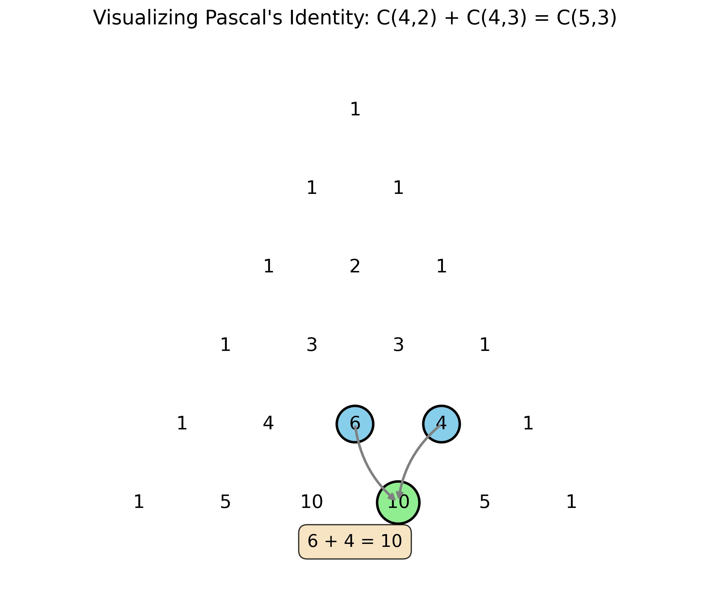
Pascal's Identity

This identity shows how the coefficients in one row of Pascal's triangle are formed from the row above it.

Theorem 5: Pascal's Identity

Let $n$ and $k$ be positive integers with $1 \leq k \leq n$. Then [1]:

\binom{n+1}{k} = \binom{n}{k-1} + \binom{n}{k}

Integration Techniques

Integration is a core concept in calculus, often used to find the area under probability density functions to calculate probabilities.

Integration by Substitution

Used when an integrand contains a function and its derivative.

Example 19: Basic Substitution

Evaluate $\int 2x \cos(x^2) \, dx$.

Let $u = x^2$, so $du = 2x \, dx$.

\int \cos(u) \, du = \sin(u) + C = \sin(x^2) + C

Example 20: More Complex Substitution

Evaluate $\int x^3 \sqrt{1-x^2} \, dx$.

Let $u = 1-x^2$. Then $du = -2x \, dx \Rightarrow x \, dx = -\frac{du}{2}$. Also, $x^2 = 1-u$.

Rewrite the integral:

\begin{align} \int x^3 \sqrt{1-x^2} \, dx &= \int x^2 \sqrt{1-x^2} \, (x \, dx) \\ &= \int (1-u) \sqrt{u} \left(-\frac{du}{2}\right) \\ &= -\frac{1}{2} \int (u^{1/2} - u^{3/2}) \, du \\ &= -\frac{1}{2} \left[\frac{u^{3/2}}{3/2} - \frac{u^{5/2}}{5/2}\right] + C \\ &= -\frac{1}{3}u^{3/2} + \frac{1}{5}u^{5/2} + C \\ &= \frac{1}{5}(1-x^2)^{5/2} - \frac{1}{3}(1-x^2)^{3/2} + C \end{align}

Method of Partial Fractions

Used to integrate rational functions (a polynomial divided by another).

Example 21: Simple Partial Fraction Decomposition

Decompose $\dfrac{5x-3}{(x+1)(x-3)}$.

\frac{5x-3}{(x+1)(x-3)} = \frac{A}{x+1} + \frac{B}{x-3}

Clear the denominator: $5x-3 = A(x-3) + B(x+1)$.

Let $x=3$: $5(3)-3 = A(0) + B(3+1) \Rightarrow 12 = 4B \Rightarrow B=3$
Let $x=-1$: $5(-1)-3 = A(-1-3) + B(0) \Rightarrow -8 = -4A \Rightarrow A=2$

So, $\dfrac{5x-3}{(x+1)(x-3)} = \dfrac{2}{x+1} + \dfrac{3}{x-3}$

Example 22: Partial Fractions with Repeated/Irreducible Roots

Decompose $\dfrac{-2x+4}{(x^2+1)(x-1)^2}$.

The form includes a linear term for the irreducible quadratic $(x^2+1)$ and terms for the repeated root $(x-1)$.

\frac{-2x+4}{(x^2+1)(x-1)^2} = \frac{Ax+B}{x^2+1} + \frac{C}{x-1} + \frac{D}{(x-1)^2}

After clearing the denominator and equating coefficients:

$A=2$
$B=1$
$C=-2$
$D=1$

So, $\dfrac{-2x+4}{(x^2+1)(x-1)^2} = \dfrac{2x+1}{x^2+1} - \dfrac{2}{x-1} + \dfrac{1}{(x-1)^2}$

Example 23: Integration with Partial Fractions

Evaluate $\displaystyle \int \frac{x+4}{x^3+3x^2-10x} \, dx$.

1. Factor denominator: $x(x^2+3x-10) = x(x+5)(x-2)$.

2. Set up fractions:

\frac{x+4}{x(x+5)(x-2)} = \frac{A}{x} + \frac{B}{x+5} + \frac{C}{x-2}

3. Solve for A, B, C (Cover-up Method):

For A (cover x, plug in x=0): $A = \dfrac{0+4}{(0+5)(0-2)} = \dfrac{4}{-10} = -\dfrac{2}{5}$
For B (cover x+5, plug in x=-5): $B = \dfrac{-5+4}{(-5)(-5-2)} = \dfrac{-1}{(-5)(-7)} = -\dfrac{1}{35}$
For C (cover x-2, plug in x=2): $C = \dfrac{2+4}{(2)(2+5)} = \dfrac{6}{14} = \dfrac{3}{7}$

4. Integrate:

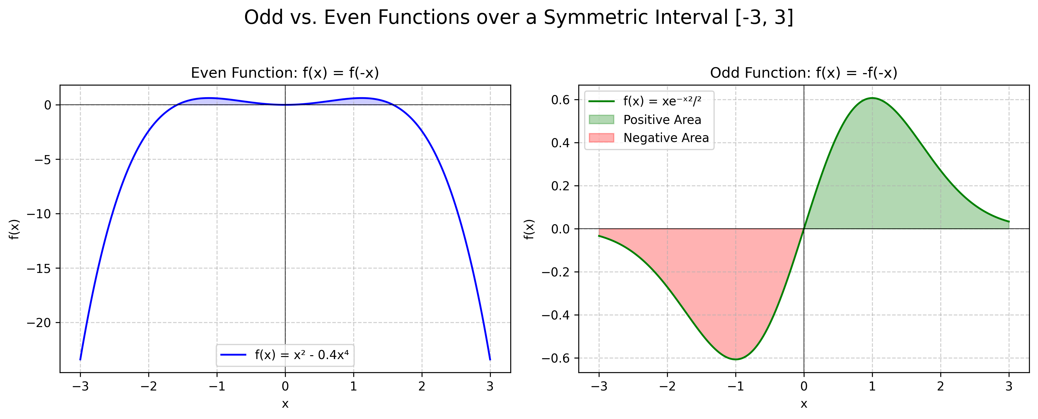
\begin{align} \int \left(-\frac{2}{5x} - \frac{1}{35(x+5)} + \frac{3}{7(x-2)}\right) dx &= -\frac{2}{5}\ln|x| - \frac{1}{35}\ln|x+5| + \frac{3}{7}\ln|x-2| + C \end{align}

Odd and Even Functions

This is a simplification for integrals over symmetric intervals, like $\int_{-a}^{a} f(x) \, dx$ [1].

An even function is symmetric about the y-axis, where $f(x) = f(-x)$. $\int_{-a}^{a} f(x) \, dx = 2 \int_{0}^{a} f(x) \, dx$
An odd function is anti-symmetric, where $f(x) = -f(-x)$. $\int_{-a}^{a} f(x) \, dx = 0$

Example 24: Odd Function

$f(x) = x e^{-x^2/2}$ is odd, since $f(-x) = (-x)e^{-(-x)^2/2} = -xe^{-x^2/2} = -f(x)$.

Therefore, $\displaystyle \int_{-5}^{5} x e^{-x^2/2} \, dx = 0$.

Odd vs. Even functions over a symmetric interval

Completing the Square

Used to transform quadratic forms into standard integral forms.

Example 25: $\arctan$ form

Evaluate $\displaystyle \int \frac{dx}{4x^2+4x+2}$.

Complete the square on the denominator:

\begin{align} 4x^2+4x+2 &= 4(x^2+x) + 2 \\ &= 4\left(x^2+x+\frac{1}{4}\right) - 1 + 2 \\ &= 4\left(x+\frac{1}{2}\right)^2 + 1 = (2x+1)^2 + 1 \end{align}

The integral becomes $\displaystyle \int \frac{dx}{(2x+1)^2 + 1}$. Let $u = 2x+1$, $du = 2 \, dx \Rightarrow dx = \dfrac{du}{2}$.

\int \frac{du/2}{u^2 + 1} = \frac{1}{2} \int \frac{du}{u^2+1} = \frac{1}{2}\arctan(u) + C = \frac{1}{2}\arctan(2x+1) + C

Example 26: $\arcsin$ form

Evaluate $\displaystyle \int \frac{dx}{\sqrt{2x-x^2}}$.

Complete the square on the denominator:

\begin{align} 2x-x^2 &= -(x^2-2x) \\ &= -(x^2-2x+1-1) \\ &= -((x-1)^2 - 1) = 1 - (x-1)^2 \end{align}

The integral becomes $\displaystyle \int \frac{dx}{\sqrt{1-(x-1)^2}}$. Let $u = x-1$, $du = dx$.

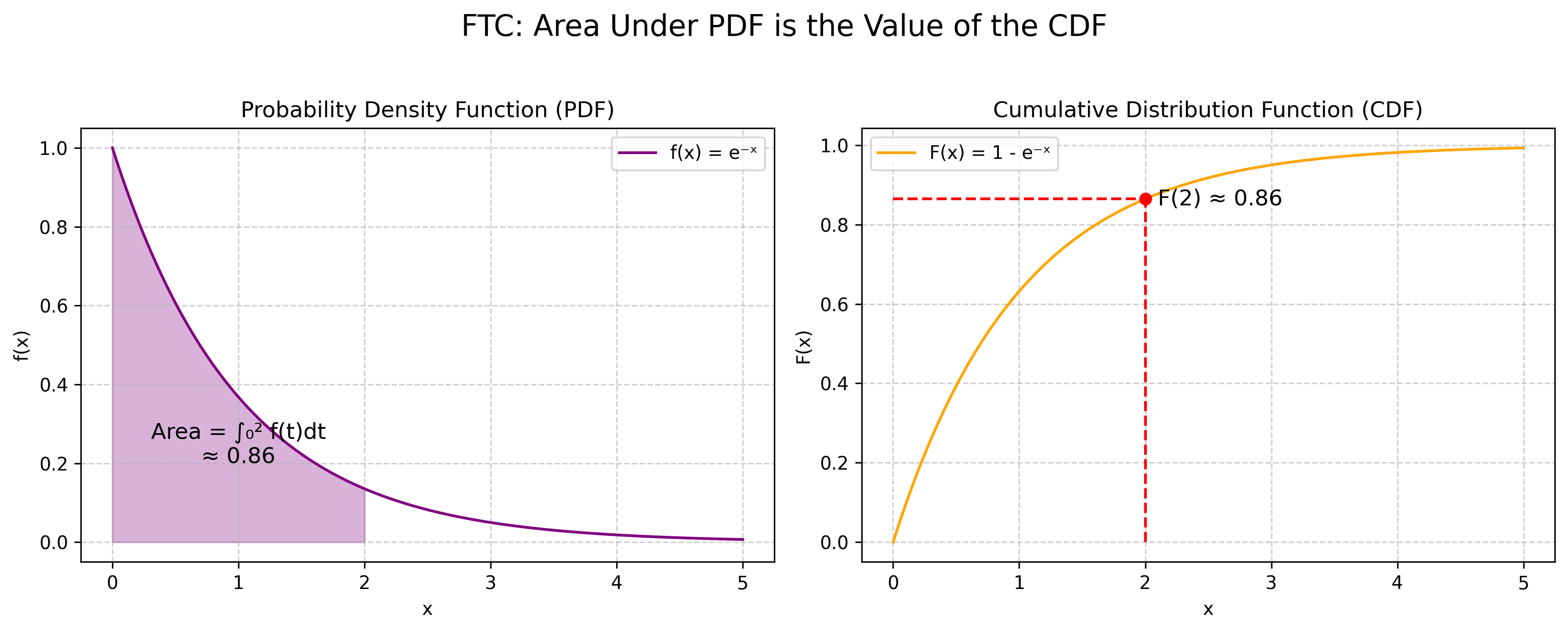
\int \frac{du}{\sqrt{1-u^2}} = \arcsin(u) + C = \arcsin(x-1) + C

The Fundamental Theorem of Calculus

The FTC links integration and differentiation, and is the formal basis for the relationship between a Probability Density Function (PDF) and a Cumulative Distribution Function (CDF) [1].

Theorem 6: Fundamental Theorem of Calculus

Let $f$ be a continuous function on $[a, b]$ [1].

f(x) = \frac{d}{dx} \int_{a}^{x} f(t) \, dt

Example 27: Demonstrating the FTC

Consider $f(t) = t^2$.

The integral from 0 to $x$ is $\displaystyle F(x) = \int_{0}^{x} t^2 \, dt = \left[\frac{t^3}{3}\right]_{0}^{x} = \frac{x^3}{3}$.

The derivative of $F(x)$ is $\displaystyle F'(x) = \frac{d}{dx}\left(\frac{x^3}{3}\right) = x^2$, which is $f(x)$.

Illustration of the FTC via a PDF and CDF — Illustration of the FTC via a PDF $f(x)$ and its CDF $\displaystyle F(x) = \int_{0}^{x} f(t) \, dt$

The Gaussian Integral

A famous definite integral that is central to probability and the normal distribution.

I = \int_{-\infty}^{\infty} e^{-x^2} \, dx = \sqrt{\pi}

Proof (using Polar Coordinates)

Square the integral and use different dummy variables: $I^2 = \left(\int_{-\infty}^{\infty} e^{-x^2} \, dx\right)\left(\int_{-\infty}^{\infty} e^{-y^2} \, dy\right) = \int_{-\infty}^{\infty} \int_{-\infty}^{\infty} e^{-(x^2+y^2)} \, dx \, dy$
Convert to polar coordinates: $x^2 + y^2 = r^2$ and $dx \, dy = r \, dr \, d\theta$. The region (entire xy-plane) becomes $r \in [0, \infty)$ and $\theta \in [0, 2\pi)$. $I^2 = \int_{0}^{2\pi} \left(\int_{0}^{\infty} e^{-r^2} r \, dr\right) d\theta$
Solve the inner integral with substitution $(u = r^2, \, du = 2r \, dr \Rightarrow r \, dr = \frac{du}{2})$: $\int_{0}^{\infty} e^{-r^2} r \, dr = \int_{0}^{\infty} e^{-u} \frac{du}{2} = \frac{1}{2} \left[-e^{-u}\right]_{0}^{\infty} = \frac{1}{2} (0 - (-1)) = \frac{1}{2}$
Solve the outer integral: $I^2 = \int_{0}^{2\pi} \frac{1}{2} \, d\theta = \frac{1}{2} \left[\theta\right]_{0}^{2\pi} = \frac{1}{2} (2\pi) = \pi$

Since $I^2 = \pi$, we have $I = \sqrt{\pi}$.

Generalized Gaussian Integral

A more general form used in statistics is:

\int_{-\infty}^{\infty} e^{-\alpha x^2} \, dx = \sqrt{\frac{\pi}{\alpha}}

Back to Notebook Index